Start with the essentials
First, learn frequency, wavelength and echo delay. Then use the worked examples before opening the deeper mathematics. You do not need a background in physics.
ACP science learning resource · Explore, listen, calculate
Sound waves. Returning echoes. A remarkable way to sense the world.
Explore how bat echolocation works, why calls change, and what a recording can really tell you. Move from sound physics to biological sonar, then test the ideas with calculators, scientific diagrams and authentic recordings.
Choose your learning route
Acoustics studies how sound starts, travels through materials and reaches a receiver. Bat acoustics connects that physics with an animal’s behaviour and hearing. However, a microphone records sound at one position, not the bat’s complete sensory experience.
First, learn frequency, wavelength and echo delay. Then use the worked examples before opening the deeper mathematics. You do not need a background in physics.
Compare detector methods, listen to field recordings with source credits and examine call shape, harmonics and recording limitations.
Explore Fourier analysis, uncertainty, classification performance and reproducibility. The advanced panels also show derivations, while keeping the main explanation easy to follow.
This is a learning guide, not a detector identification key or a replacement for a survey of your site. The British bats guide covers anatomy, species and ecology. Our bat survey service explains the route from project questions to suitable evidence.
Connect the disciplines
Physical acoustics explains waves, reflection and energy transfer. Architectural acoustics also studies sound in and around buildings, including repeated reflections and reverberation. For example, a façade, tunnel or roof can alter the sound arriving at a detector.
Bioacoustics studies how animals make, hear and use sound. Psychoacoustics studies how physical sound relates to what a listener perceives. However, human loudness judgements cannot simply be transferred to a bat’s auditory system.
Environmental acoustics describes sources, paths and receivers in real settings. Ultrasonics concerns frequencies above ordinary human hearing. Signal analysis then turns a sampled waveform into measurements while preserving its context and uncertainty.
A useful review follows the whole chain: source → propagation → microphone → processing → interpretation. A changed recording may reflect a changed call, a different flight angle, weather, equipment or analysis settings. First, work out which of these causes may apply.
Evidence: Goerlitz (2018), weather, attenuation and monitoring · OpenStax, University Physics volume 1, §§17.1–17.3.
The physical foundations
A vibrating source pushes and pulls the surrounding air. Nearby particles compress and separate, passing the disturbance to their neighbours. The pattern travels, but each air particle mainly moves back and forth around its rest, or equilibrium, position.
In air and water, small-amplitude sound is a longitudinal pressure wave. Solids can also support shear waves. Because mechanical motion needs matter, sound does not travel through a vacuum. Its speed depends on the medium’s stiffness and density; the same frequency can therefore have different wavelengths in air and water.
Frequency f counts cycles per second, in hertz. Period T is the time for one cycle, in seconds. Wavelength λ is the distance between matching points in successive cycles. Sound speed c links time and distance.
f: hertz (Hz); T: seconds (s); λ: metres (m); c: metres per second (m/s).
 © 2026 ACP Consultants Ltd. · Original educational diagram
Evidence: OpenStax, University Physics volume 1, §§17.1–17.3 · OpenStax, speed of sound.
Laboratory 01 · wavelength & distance
At an example sound speed of 343 m/s, a 1 kHz wave has a wavelength of 343 mm. At 45 kHz it is 7.62 mm; at 55 kHz it is 6.24 mm. Higher frequency means more cycles within the same distance, when sound speed stays constant.
Wavelength affects diffraction and scattering. For example, objects much smaller than a wavelength can scatter weakly, but there is no single wavelength-sized cut-off for detection. Target shape, orientation, returning energy and the animal’s hearing also matter.
θ is air temperature in °C. We use this approximate dry-air relationship over −10 to 35°C here; it omits humidity, pressure changes and wind gradients.
The tool uses this temperature approximation rather than fixing c at 343 m/s. Consequently, at 20°C it reports 343.42 m/s and a slightly different wavelength. That small difference reflects the stated assumptions, not a conflict.
Try 1 kHz, then 45 kHz. Next, keep distance unchanged: the geometrical spreading result stays the same because this ideal model excludes frequency-dependent absorption.
Spherical free-field spreading only. Reference distance 1 m; no atmospheric absorption or obstacles. Not a species detection-distance predictor.
© 2026 ACP Consultants Ltd. · Original educational diagramEvidence: OpenStax, University Physics volume 1, §§17.1–17.3 · Goerlitz (2018), weather, attenuation and monitoring.
A model with explicit assumptions
The simplest model is a harmonic pressure change around ambient pressure. Its amplitude sets the peak pressure change, while phase shifts where the oscillation starts. Frequency then sets how quickly the trace repeats.
p′ is pressure deviation in Pa; A is peak pressure amplitude in Pa; f is Hz; t is s; φ is phase in radians.
In contrast, a real bat call changes in frequency and amplitude over time. It may contain several harmonics, because the sound-producing structure is not a perfect sinusoidal oscillator. Bandwidth describes the frequency span under a stated measurement rule.
Superposition means small disturbances add. Two identical waves can reinforce when in phase or cancel at a location when opposite in phase. However, cancellation at one point does not mean the acoustic energy has vanished everywhere.
Pressure: a local fluctuation, measured in pascals.
Intensity: average energy flow per unit area, measured in W/m².
Power: total acoustic energy emitted per unit time, measured in watts.
For a progressive plane wave, I = p²rms/(ρ₀c). Here ρ₀ is mean density in kg/m³. However, check the conditions before using this relationship in a reactive near field or standing wave.
© 2026 ACP Consultants Ltd.For an inviscid fluid initially at rest, linearised momentum gives ρ₀ ∂u/∂t = −∇p′. Linearised mass conservation gives ∂ρ′/∂t = −ρ₀∇·u. With a small, nearly adiabatic disturbance, p′ = c²ρ′.
Differentiate the pressure–density relation in time, substitute mass conservation, and differentiate again. Substitution of the momentum equation then gives:
u is particle velocity (m/s); ρ′ is density perturbation (kg/m³); ∇ is the spatial gradient and ∇² the Laplacian (inverse-square length). Both sides have units Pa/s².
This derivation assumes small changes, uniform equilibrium properties and no source term in the region being studied. It omits viscosity, thermal losses, boundaries and background flow. For an outdoor scene, check how well these conditions apply.
Evidence: OpenStax, University Physics volume 1, §§17.1–17.3.
Laboratory 02 · pressure & level
A decibel is a logarithmic ratio. Sound pressure level in air compares root mean square pressure with a reference of 20 micropascals. Therefore, give the reference with the number: “80 dB” alone leaves a key question unanswered.
Lp is dB re 20 µPa; prms and pref are in Pa. For air, pref = 0.000020 Pa.
A sine wave has an RMS pressure of A/√2. For example, 0.020 Pa RMS gives 20 log₁₀(1,000) = 60 dB SPL. Doubling pressure adds 6.02 dB because the logarithm contains a factor of twenty.
Intensity level uses 10 log₁₀(I/Iref). Doubling intensity adds 3.01 dB. In a progressive wave with unchanged impedance, intensity is proportional to squared RMS pressure. Thus doubling pressure quadruples intensity; these two statements agree.
For two independent, equal-level sources, add their mean-square pressures: the combined level rises by about 3 dB. However, perfectly coherent equal signals can behave differently because their relative phase matters.
RMS pressure must be a calibrated physical measurement. However, this calculation cannot calibrate a WAV file.
© 2026 ACP Consultants Ltd.Frequency weighting also changes the question. A-weighting approximates aspects of human hearing; it does not describe a bat’s sensitivity. Also, an ordinary sound-level meter may not have an ultrasonic microphone or a suitable frequency response. An environmental noise result in dB(A) cannot, by itself, measure ultrasonic exposure at a bat’s ear.
Evidence: OpenStax, sound intensity · Goerlitz (2018), weather, attenuation and monitoring.
Source → path → receiver
Sound changes along its path, even before a detector processes it. For example, spreading redistributes energy across a growing area. Atmospheric absorption converts part of that energy into heat. Reflections and scattering change the paths that reach the receiver.
Relative pressure-level change in dB for ideal spherical spreading. Both distances use the same units and lie outside the immediate source region.
For example, from 2 m to 4 m, the ideal change is −6.02 dB. From 1 m to 10 m, it is −20 dB. These are one-way spreading changes; a bat detecting an echo also faces the outward path and the target’s scattering properties.
α is atmospheric attenuation in dB/m at a stated frequency and atmospheric condition. This simplified narrowband model omits ground interference, refraction, source directivity and target effects.
Goerlitz’s analysis shows that ultrasonic attenuation depends nonlinearly on frequency, temperature, humidity and pressure. Consequently, “more humid always means more attenuation” is not a reliable general rule. Instead, use a documented model within its valid range. Do not assume a fixed loss per metre without evidence.
Reflection and reverberation: walls or water can return extra delayed paths. Smooth surfaces favour directional reflection; geometry controls whether that energy reaches a receiver.
Diffraction and scattering: edges bend the field and rough structures redistribute it. Therefore, their scale relative to wavelength matters.
Refraction: temperature and wind gradients bend sound paths through changes in effective propagation speed.
Vegetation and ground: leaves, branches and direct/reflected path interference create frequency-selective changes. Therefore, vegetation is not a uniform sound curtain.
Evidence: Goerlitz (2018), weather, attenuation and monitoring.
From pressure to perception
The outer ear collects sound and helps encode direction. The middle ear then passes vibration to the inner ear. In the cochlea, mechanical filtering and sensory cells convert vibration into neural signals. The brain interprets those signals in time and context.
The familiar human range of roughly 20 Hz–20 kHz is a rough guide, often describing young listeners under suitable conditions. Thresholds vary with frequency, age, individual and sound level. Infrasound and ultrasound describe frequencies below and above this usual range, not absolute boundaries between “sound” and “no sound”.
Frequency relates to pitch, while perceived loudness depends on level, spectrum, duration and hearing. A graph of pressure amplitude is therefore not a complete account of what an animal perceives.
British bats often use ultrasonic echolocation, but social sounds and some lower-frequency call components can be audible to people. Horseshoe bats have specialised narrowband auditory processing; this should not be assumed to apply to every bat. Long-eared bats can also listen for prey-generated sounds.
© 2026 ACP Consultants Ltd.Evidence: Denzinger & Schnitzler (2013), bat guilds and echolocation · BCT, UK bats and species accounts.
Laboratory 03 · biological sonar
British bats produce echolocation calls using the larynx and emit them through the mouth or nostrils. The emitted beam illuminates only part of the surroundings. As a result, returning echoes depend on the objects within that beam and the direction of reflection.
The simplest ranging cue is delay. Sound travels from bat to target and back, so the path is twice the target distance. Therefore, divide round-trip travel time by two when converting it to distance.
d is one-way target distance (m); c is sound speed (m/s); Δt is round-trip delay (s).
At 343 m/s, a target 3 m away produces a delay of 2 × 3/343 = 0.01749 s, or 17.5 ms. However, omitting the factor of two would place it at 6 m.
Several reflectors create several echoes. Target motion, changing sound speed and overlapping calls complicate the scene. Direction, spectrum, amplitude and changes from one echo to the next add clues. The animation below shows travel time; it does not recreate what a bat perceives.
For a simple pulse-and-echo example, a 10 m path to a target takes about 58.3 ms for the round trip at 343 m/s. If the bat emits another call before a distant echo returns, matching echoes to calls becomes harder. However, real bats use sequences and multiple cues; the single-pulse diagram does not model that processing.
Stationary bat and target; straight path and constant sound speed. However, changing frequency changes wavelength, not the delay in this model. No sound is played. Reduced-motion settings suppress animation.
© 2026 ACP Consultants Ltd. · Original educational diagramEvidence: Denzinger & Schnitzler (2013), bat guilds and echolocation · OpenStax, speed of sound.
Laboratory 04 · calls in motion
Doppler shift arises when source and receiver move relative to the medium. An approaching source compresses the spacing of arriving wavefronts. An approaching receiver encounters them more rapidly. Therefore, state the geometry before choosing an equation.
One-dimensional still-air convention: vr is receiver speed towards the source; vs is source speed towards the receiver. Speeds are m/s and positive for approach. f0 and fr are in Hz.
A stationary detector receiving a 45 kHz tone from a source approaching at 5 m/s, with c = 343 m/s, measures about 45.67 kHz. However, that one-way example is not the same as a returning echo.
For a bat moving towards a stationary reflector, first treat the bat as a moving source. Then treat the bat as a moving receiver of the reflected wave. In this simplified straight-line geometry:
fe is received echo frequency; v is bat speed towards a stationary reflector. Here, we assume that the reflector does not change frequency in the medium frame.
At 5 m/s and 45 kHz, the echo is about 46.33 kHz: a 1.33 kHz increase. For speeds much smaller than c, Δf ≈ 2f₀v/c. However, wingbeat motion and oblique flight need more detailed treatment.
Sound speed fixed at 343 m/s. Negative speed means recession. A pure-tone teaching model; no species identification or flight-speed estimate from an unknown call.
© 2026 ACP Consultants Ltd.Evidence: OpenStax, the Doppler effect · Denzinger & Schnitzler (2013), bat guilds and echolocation.
Form follows behaviour
Open-space calls can be relatively long and shallow in frequency modulation. In clutter, a bat may shorten calls and broaden their sweep to separate nearby echoes. The same bat therefore changes its output as the task changes.
As a target becomes close, intervals between calls often shorten. For example, a terminal feeding buzz can provide rapid updates during a capture attempt. However, it does not prove that the prey was caught, swallowed or identified.
In addition, social calls can contain varied syllables, repeated phrases and harmonics. Their function depends on timing, behaviour and interactions. Some social components are high-frequency; “social” does not simply mean “low-pitched”.
Frequency modulation (FM) describes a sweep; quasi-constant frequency (QCF) describes a fairly shallow segment; constant frequency (CF) describes a sustained narrowband component. However, these describe structure, not mutually exclusive species labels. Indeed, a single call can combine components.
© 2026 ACP Consultants Ltd. · Original educational diagramEvidence: Denzinger & Schnitzler (2013), bat guilds and echolocation · Götze, Denzinger & Schnitzler (2020), calls and flight behaviour.
Keep the ecological context
First, state which call parameter you are measuring. Peak frequency, frequency of maximum energy, end frequency and a detector’s best listening setting do not all mean the same thing. A spectrogram’s strongest bin can also change with the selected pulse, analysis window and recording geometry.
| Group or species | What to compare | Why caution is needed |
|---|---|---|
| Common, soprano & Nathusius’ pipistrelles | FM–QCF shape, tail/peak region, duration and whole sequence. “45” and “55 kHz” are familiar common/soprano shorthand. | Frequency changes with flight and habitat; Nathusius’ overlaps lower-frequency pipistrelle calls. Use current reference accounts. |
| Noctule, Leisler’s & serotine | Lower-frequency search calls; slope, alternating calls, duration and intervals. | Open-space calls can overlap. The noctule example below has strong components around 18–20 kHz, not a fixed species boundary. |
| Greater & lesser horseshoes | Long narrowband components and FM edges; identify the harmonic being compared. | The examples below show components near 82 and 110 kHz. Geographical and individual variation, Doppler and equipment response matter. |
| Myotis species | Broadband steep FM sweeps, sequence, habitat and corroboration. | Several British species overlap strongly; a confident species-level label may not be justified. |
| Brown & grey long-eared bats | Weak, broadband signals, harmonic structure and independent evidence. | Quiet or off-axis calls can be missed. These species are not reliably separated by a simple sound match. |
| Barbastelle | Short calls, call-type sequence and frequency structure. | Direction, noise and missing calls can obscure the pattern. Use a reviewed sequence, not one isolated pulse. |
Start and end frequency depend on the amplitude threshold used to define the visible call. Duration also changes if a weak onset falls below that threshold. Therefore, record the measurement rule, not just the resulting number. When evidence supports only a group, report the group.
Our British bat species profiles cover all 18 species. Use them for anatomy, seasonal behaviour and further listening examples. Here, the advanced library selects contrasting call structures rather than repeating the whole identification guide.
Evidence: BCT, UK bats and species accounts · Goerlitz (2018), weather, attenuation and monitoring · Perks, O’Connell & Goodenough (2026), classifier comparisons.
The conversion matters
Frequencies must use the same units.
Mixing a 45 kHz signal with a 40 kHz oscillator produces a 5 kHz difference component. It also produces a higher-frequency sum component, which is usually filtered out. The listening band depends on tuning. However, the output does not preserve the whole original ultrasonic spectrum.
N is the division ratio.
Division by ten moves a 45 kHz component to 4.5 kHz while broadly retaining live timing. Traditional zero-crossing systems retain less amplitude and harmonic detail than a full-spectrum waveform. Therefore, they are not simply a slowed high-fidelity recording.
k is the expansion factor.
At tenfold expansion, 45 kHz becomes 4.5 kHz and a 5 ms call lasts 50 ms. Both pitch and duration change. However, some traditional devices cannot record while replaying; continuous full-spectrum systems and listening modes differ.
A suitable ultrasonic microphone and recorder sample pressure-related voltage at a high enough rate. That waveform supports later filtering and spectral analysis. However, it is still shaped by microphone response, orientation, gain, electronics and triggering.
Zero-crossing records instead retain timing data about crossings or derived frequency tracks. They can be compact and useful, but missing amplitude data cannot be restored by drawing a colourful spectrogram.
Evidence: BCT, detector methods.
Laboratory 05 · hear the method
For example, use one hypothetical 45 kHz, 5 ms call. Time expansion and frequency division can give the same stated 4.5 kHz output frequency, but the output durations differ. In contrast, heterodyne output depends on the tuning frequency.
The full-spectrum option reports the original signal rather than pretending it is audible. This tool changes numbers and a schematic; it does not produce ultrasound or claim to reproduce the full behaviour of a detector circuit.
In heterodyne mode, an incoming component above the reference and one equally far below it can produce the same difference frequency. Therefore, without the tuning setting, that audible component cannot by itself reveal the original ultrasonic frequency.
A call also sweeps through the listening band. Only part of its trajectory may be audible, so changing the reference can alter its apparent texture. For quantitative analysis, preserve the original full-spectrum signal where available.
A pure-tone model. Real bat calls contain time-varying frequency and amplitude; detector bandwidth and filtering are not simulated.
© 2026 ACP Consultants Ltd. · Original educational diagramEvidence: BCT, detector methods.
Avoid confident measurements of damaged data
Sampling records values at regular intervals. A sample rate fs gives a Nyquist frequency of fs/2. However, signal energy above that boundary can fold into lower frequencies unless a suitable anti-alias filter removes it before sampling.
fs and fmax are in Hz. In practice, strict inequality and transition-band margin matter; this is not permission to assume an ideal real-world filter.
A 384 ksample/s recorder has a theoretical Nyquist limit of 192 kHz. However, that does not guarantee flat sensitivity up to 192 kHz. A 48 ksample/s recorder has a 24 kHz Nyquist limit; a 50 kHz input could alias to 2 kHz in an ideal unfiltered sampling example.
To capture useful content to 120 kHz, the theoretical boundary is 240 ksample/s. However, real equipment also needs extra margin, enough microphone bandwidth and a suitable anti-alias design. Inspect the complete recording chain.
Frequency response: confirm microphone and recorder bandwidth, not just sample rate.
Gain and clipping: flat-topped peaks indicate saturation. Lowering playback volume cannot restore clipped data.
Bit depth: more quantisation levels can show finer amplitude changes, but microphone self-noise may dominate.
Trigger settings: threshold, pre-trigger buffer and maximum file length affect which calls are retained.
Time and placement: synchronised clocks, orientation, height and weather records make comparison meaningful.
For a uniform b-bit quantiser and a full-scale sine wave, an idealised signal-to-quantisation-noise ratio is about 6.02b + 1.76 dB. At 16 bits this gives about 98.1 dB. The result assumes ideal quantisation noise and a stated full-scale convention.
However, this is not the acoustic dynamic range of an installed bat detector. Analogue noise, microphone sensitivity, gain, frequency response and interference can dominate. Keep raw source files rather than exporting only compressed listening copies.
Evidence: BCT, detector methods · SciPy, ShortTimeFFT documentation.
From samples to interpretable evidence
Pressure-related sample amplitude against time. Use it to locate events, inspect clipping and see the envelope. However, rapid oscillations can be unreadable when zoomed out; an envelope is not a frequency measurement.
Frequency content over a chosen interval. It helps locate components but does not show when they occur within that interval. A whole-file peak can belong to background noise rather than the pulse of interest.
Repeated windowed spectra arranged across time. The horizontal axis is time, the vertical axis frequency, and colour shows a stated magnitude or power scale. Therefore, it is an analysis product, not a photograph of sound.
A discrete Fourier transform compares a finite sample sequence with sinusoidal components. The transform then returns complex coefficients, which contain amplitude and phase information. A short-time Fourier transform repeats the calculation across overlapping windows.
x[n] is the sampled signal; n is sample index; N is transform length; k is frequency-bin index; i² = −1. Bin frequency is kfs/N Hz.
m is frame index; H is hop size in samples; w[n] is the window. The window selects and weights each short segment.
At fs = 384 ksample/s and N = 512, bin spacing is 750 Hz and window duration is 1.33 ms. With N = 2,048, spacing is 187.5 Hz and duration is 5.33 ms.
The longer window narrows bin spacing but blends a longer interval. As a result, a rapidly changing call can become blurred in time. In contrast, a shorter window follows changes better but separates nearby frequencies less sharply.
However, bin spacing is not identical to true resolving power. Window shape and signal structure matter. Zero-padding makes the sampled display denser without adding new data.
A Hann window tapers the ends of a segment, reducing leakage from discontinuities. It also broadens the main lobe relative to a rectangular window. Therefore, compare like with like when reporting measured bandwidth or peak frequency.
Magnitude displays commonly use 20 log₁₀(|X|/Xref); power displays use 10 log₁₀(P/Pref). Therefore, state the reference, window correction, scaling and any floor. A colour scale normalised to the largest component in one figure cannot be compared directly with a differently normalised figure.
Report the original sample rate, channel, selected interval, FFT/window length, hop, window function, frequency band and threshold used for start/end measurements. Also keep enough detail so another analyst can produce the same plot.
Evidence: SciPy, ShortTimeFFT documentation · Goerlitz (2018), weather, attenuation and monitoring.
Laboratory 06 · time–frequency trade-off
This explorer analyses a synthetic 80-to-30 kHz downward sweep lasting 4 ms, repeated every 18 ms. Its sampling rate is 384 ksample/s. Next, change the Hann window length while holding the underlying signal fixed.
A short window follows the sweep’s timing. In contrast, a long window captures more oscillations but spans much of the call, spreading energy across a wider time region. The display uses actual short-time Fourier calculations on the teaching signal.
The example is deliberately simple: there is no microphone response, atmospheric loss or background noise. For comparison, real measured examples follow below. The colour scale shows relative magnitude, not calibrated sound pressure.
Synthetic teaching data, not a bat recording. Hop 128 samples; display range −50 to 0 dB relative to the strongest plotted coefficient. No zero-padding.
© 2026 ACP Consultants Ltd. · Original educational diagramEvidence: SciPy, ShortTimeFFT documentation.
Authentic audio · visible provenance
These eight examples contrast call structures and recording contexts. They are genuine attributed recordings of species found in Britain, including recordings made elsewhere in Europe. They are not ACP project recordings. The repository’s species label is stated evidence, not independent ACP confirmation.
All players are manual and use 10× slower playback. Frequency is divided by ten and duration multiplied by ten. The spectrograms retain the original time and ultrasonic frequency axes. Playback gain is normalised, so volume cannot be used to compare source level between bats.
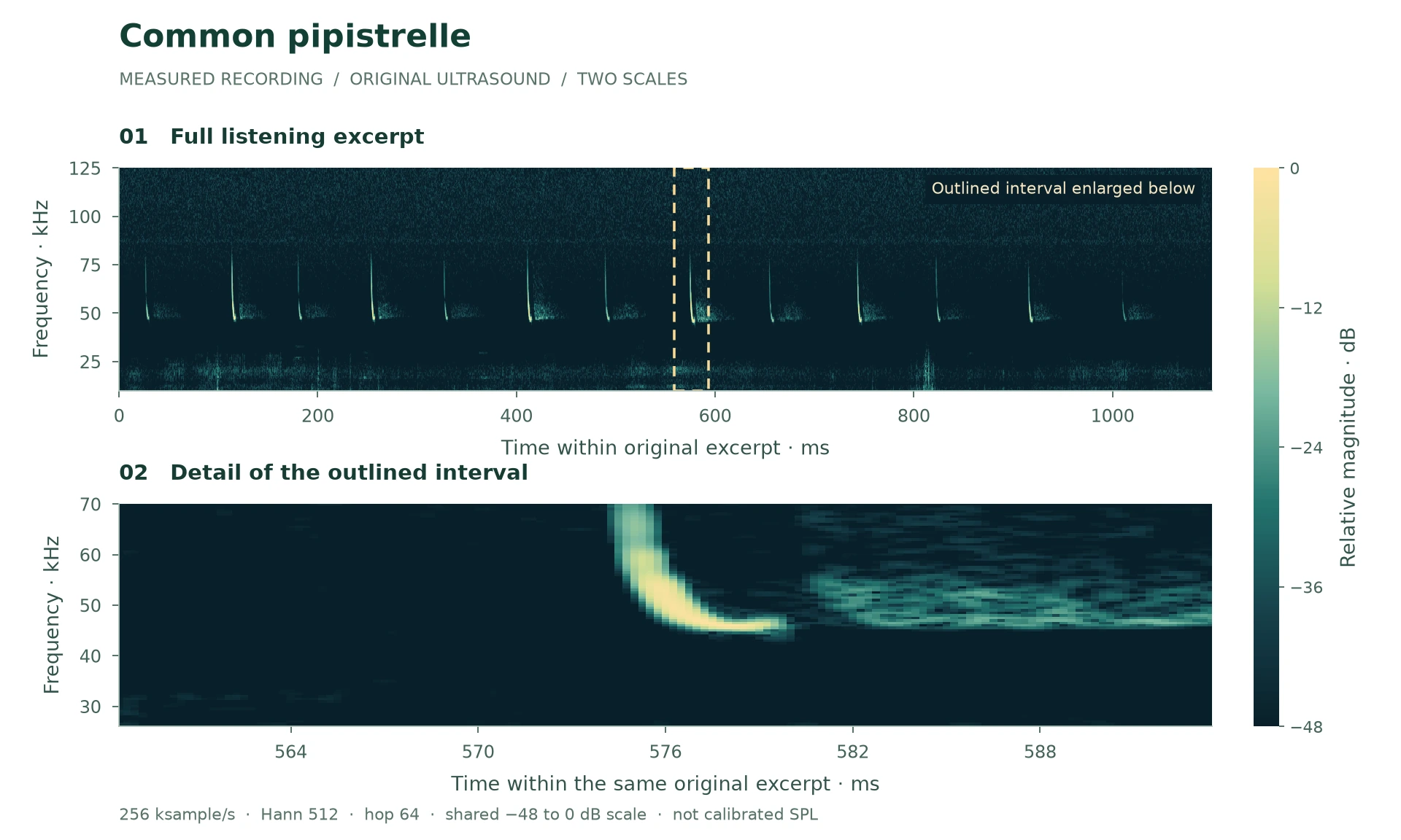
Pipistrellus pipistrellus
10× slower · 11.0 seconds
Hear regularly spaced clicks when slowed. The measured calls sweep down towards a flatter tail. This field sequence has greatest energy near 47.5 kHz within the stated analysis band; “45 kHz bat” is a shorthand, not a fixed identity test.
Recording credit: (c) Uploads from the Somerset Bat Groups events and members, some rights reserved (CC BY)
(c) Uploads from the Somerset Bat Groups events and members, some rights reserved (CC BY) · CC BY 4.0. Recorded in United Kingdom; this is not an ACP project recording. iNaturalist research; community identification, not independent ACP confirmation.
Original 256 ksample/s; channel 1. Excerpt 6.526–7.626 seconds. Playback is 10× slower, with frequency divided by ten and duration multiplied by ten. Gain was normalised, then resampled to 32 kHz for MP3. No denoising was applied.
The spectrogram uses original samples, a 512-sample Hann window and a 64-sample hop. Levels are relative to the strongest plotted component, not calibrated dB SPL. Original files and processing records are retained.
The lower plot enlarges 558.5–593.5 ms within this excerpt. It selects a high-energy interval within the documented analysis band. This is a visual teaching detail, not an independently verified species identification. Both plots use the same −48 to 0 dB reference.
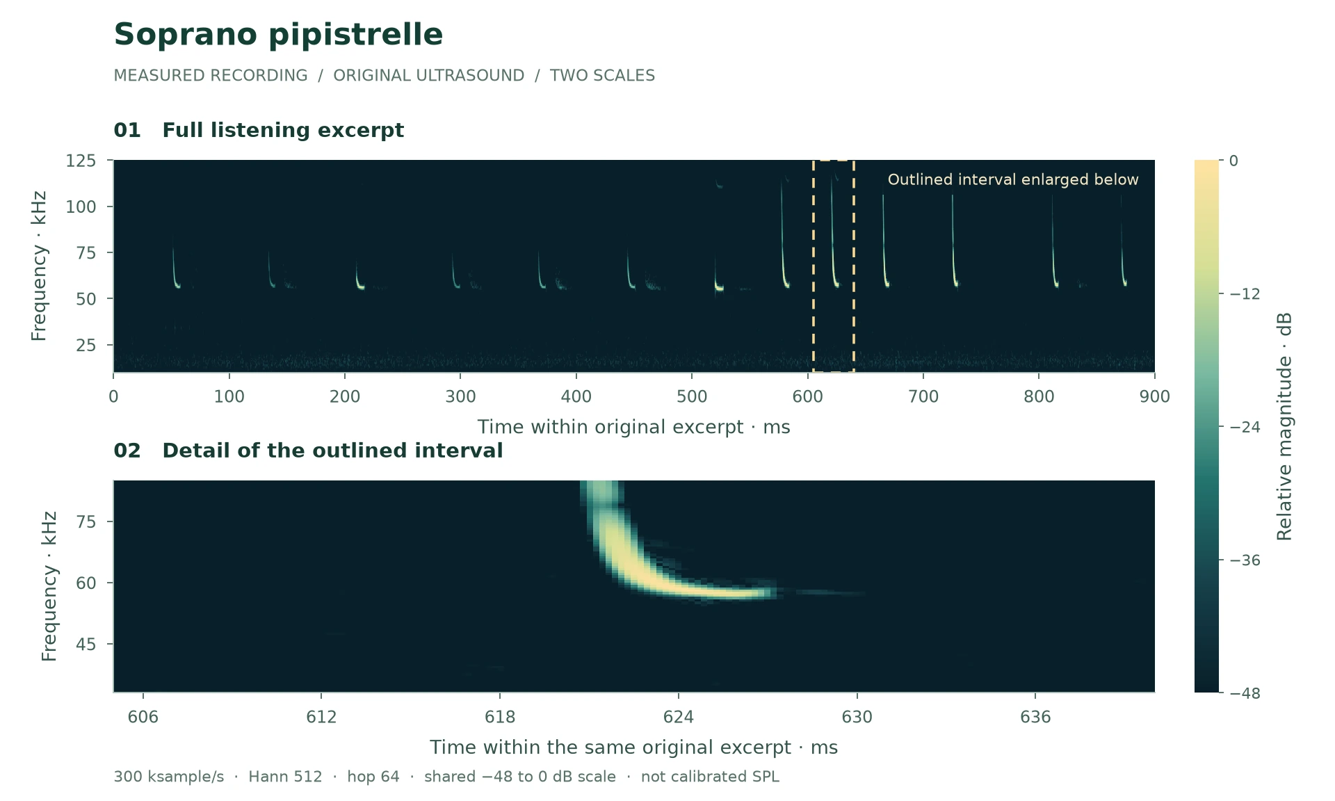
Pipistrellus pygmaeus
10× slower · 9.0 seconds
Compare these downward sweeps with the common pipistrelle example. Their lower portion sits higher on the frequency scale. This excerpt peaks near 58 kHz in the analysis band, illustrating why the familiar “55 kHz” label is approximate.
Recording credit: Jespersen, Docherty, Albertsen, Hallam & Jakobsen (2022)
Jespersen, Docherty, Albertsen, Hallam & Jakobsen (2022) · CC BY 4.0. Recorded in Denmark; this is not an ACP project recording. Species label from published research dataset; not independently confirmed by ACP.
Original 300 ksample/s; channel 3. Excerpt 5.550–6.450 seconds. Playback is 10× slower, with frequency divided by ten and duration multiplied by ten. Gain was normalised, then resampled to 32 kHz for MP3. No denoising was applied.
The spectrogram uses original samples, a 512-sample Hann window and a 64-sample hop. Levels are relative to the strongest plotted component, not calibrated dB SPL. Original files and processing records are retained.
The lower plot enlarges 605.0–640.0 ms within this excerpt. It selects a high-energy interval within the documented analysis band. This is a visual teaching detail, not an independently verified species identification. Both plots use the same −48 to 0 dB reference.
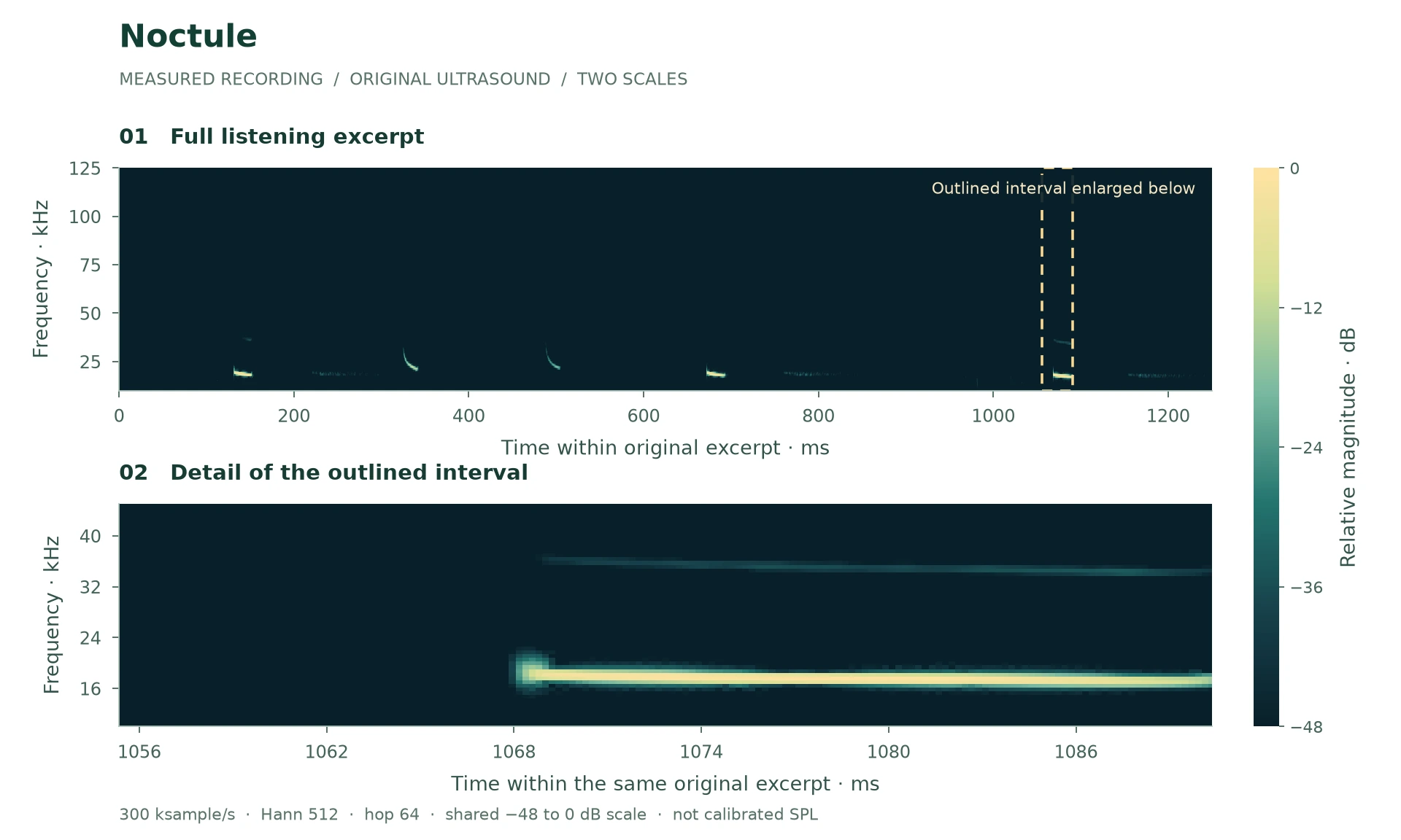
Nyctalus noctula
10× slower · 12.5 seconds
Listen for the slower rhythm and lower audible pitch. Several pulses sit near 18–20 kHz, while others sweep more strongly. A single low-frequency call still needs comparison with other open-air bats.
Recording credit: Jespersen, Docherty, Albertsen, Hallam & Jakobsen (2022)
Jespersen, Docherty, Albertsen, Hallam & Jakobsen (2022) · CC BY 4.0. Recorded in Denmark; this is not an ACP project recording. Species label from published research dataset; not independently confirmed by ACP.
Original 300 ksample/s; channel 3. Excerpt 9.350–10.600 seconds. Playback is 10× slower, with frequency divided by ten and duration multiplied by ten. Gain was normalised, then resampled to 32 kHz for MP3. No denoising was applied.
The spectrogram uses original samples, a 512-sample Hann window and a 64-sample hop. Levels are relative to the strongest plotted component, not calibrated dB SPL. Original files and processing records are retained.
The lower plot enlarges 1055.4–1090.4 ms within this excerpt. It selects a high-energy interval within the documented analysis band. This is a visual teaching detail, not an independently verified species identification. Both plots use the same −48 to 0 dB reference.
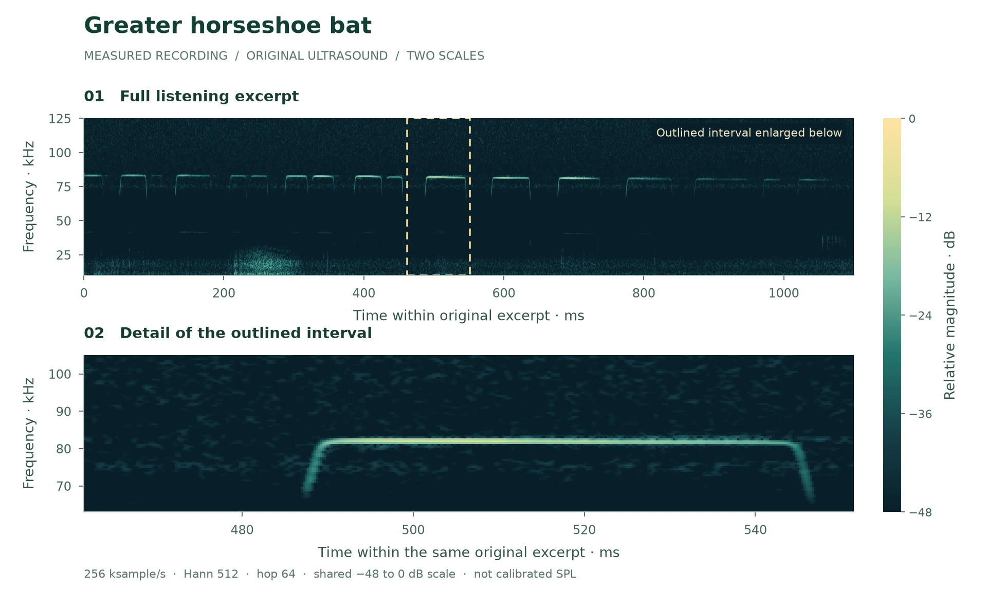
Rhinolophus ferrumequinum
10× slower · 11.0 seconds
Longer, nearly horizontal components near 82 kHz stand out in this excerpt. Short frequency-modulated edges also matter; do not compare this value with a peak measured from another harmonic.
Recording credit: (c) Uploads from the Somerset Bat Groups events and members, some rights reserved (CC BY)
(c) Uploads from the Somerset Bat Groups events and members, some rights reserved (CC BY) · CC BY 4.0. Recorded in United Kingdom; this is not an ACP project recording. iNaturalist research; community identification, not independent ACP confirmation.
Original 256 ksample/s; channel 1. Excerpt 9.493–10.593 seconds. Playback is 10× slower, with frequency divided by ten and duration multiplied by ten. Gain was normalised, then resampled to 32 kHz for MP3. No denoising was applied.
The spectrogram uses original samples, a 512-sample Hann window and a 64-sample hop. Levels are relative to the strongest plotted component, not calibrated dB SPL. Original files and processing records are retained.
The lower plot enlarges 461.5–551.5 ms within this excerpt. It selects a high-energy interval within the documented analysis band. This is a visual teaching detail, not an independently verified species identification. Both plots use the same −48 to 0 dB reference.
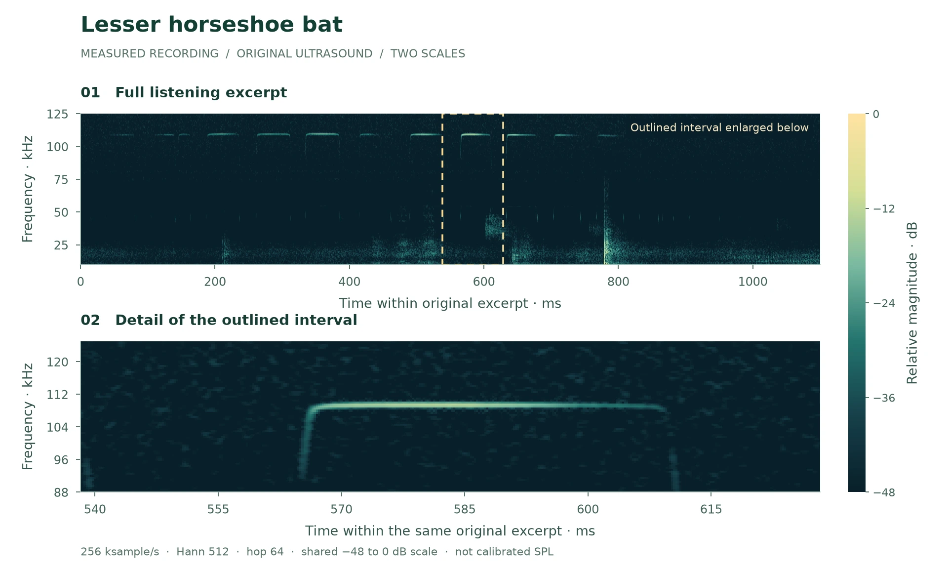
Rhinolophus hipposideros
10× slower · 11.0 seconds
The narrowband components are near 110 kHz in this recording. A detector needs sufficient ultrasonic bandwidth and sample rate to preserve them. Ordinary phone audio cannot record this band.
Recording credit: (c) Uploads from the Somerset Bat Groups events and members, some rights reserved (CC BY)
(c) Uploads from the Somerset Bat Groups events and members, some rights reserved (CC BY) · CC BY 4.0. Recorded in United Kingdom; this is not an ACP project recording. iNaturalist research; community identification, not independent ACP confirmation.
Original 256 ksample/s; channel 1. Excerpt 2.282–3.382 seconds. Playback is 10× slower, with frequency divided by ten and duration multiplied by ten. Gain was normalised, then resampled to 32 kHz for MP3. No denoising was applied.
The spectrogram uses original samples, a 512-sample Hann window and a 64-sample hop. Levels are relative to the strongest plotted component, not calibrated dB SPL. Original files and processing records are retained.
The lower plot enlarges 538.2–628.2 ms within this excerpt. It selects a high-energy interval within the documented analysis band. This is a visual teaching detail, not an independently verified species identification. Both plots use the same −48 to 0 dB reference.
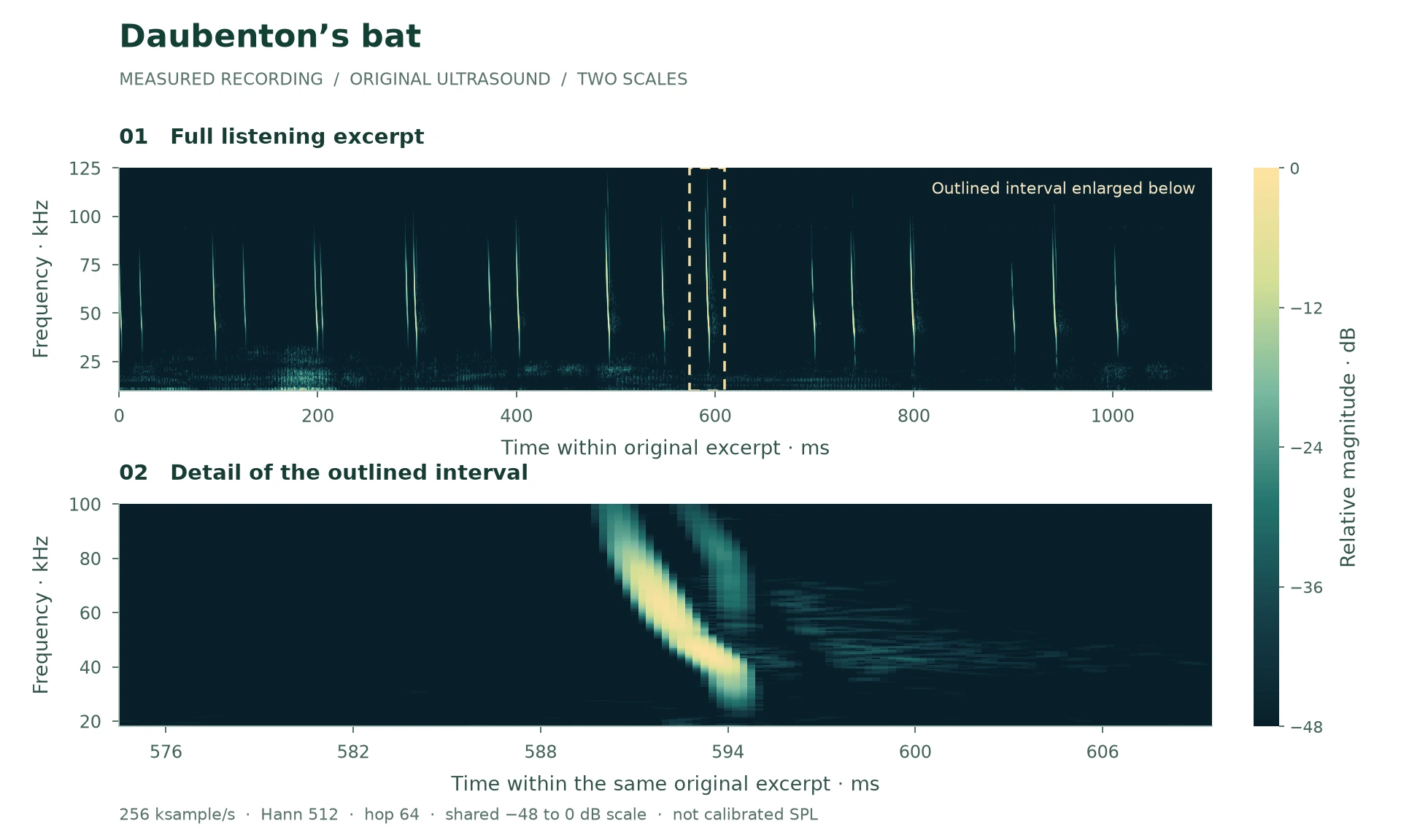
Myotis daubentonii
10× slower · 11.0 seconds
Steep frequency sweeps are visible. The source identifies Daubenton’s bat, but similar Myotis calls overlap. Acoustic shape must be considered with recording context and independent evidence.
Recording credit: (c) Uploads from the Somerset Bat Groups events and members, some rights reserved (CC BY)
(c) Uploads from the Somerset Bat Groups events and members, some rights reserved (CC BY) · CC BY 4.0. Recorded in United Kingdom; this is not an ACP project recording. iNaturalist research; community identification, not independent ACP confirmation.
Original 256 ksample/s; channel 1. Excerpt 1.822–2.922 seconds. Playback is 10× slower, with frequency divided by ten and duration multiplied by ten. Gain was normalised, then resampled to 32 kHz for MP3. No denoising was applied.
The spectrogram uses original samples, a 512-sample Hann window and a 64-sample hop. Levels are relative to the strongest plotted component, not calibrated dB SPL. Original files and processing records are retained.
The lower plot enlarges 574.5–609.5 ms within this excerpt. It selects a high-energy interval within the documented analysis band. This is a visual teaching detail, not an independently verified species identification. Both plots use the same −48 to 0 dB reference.
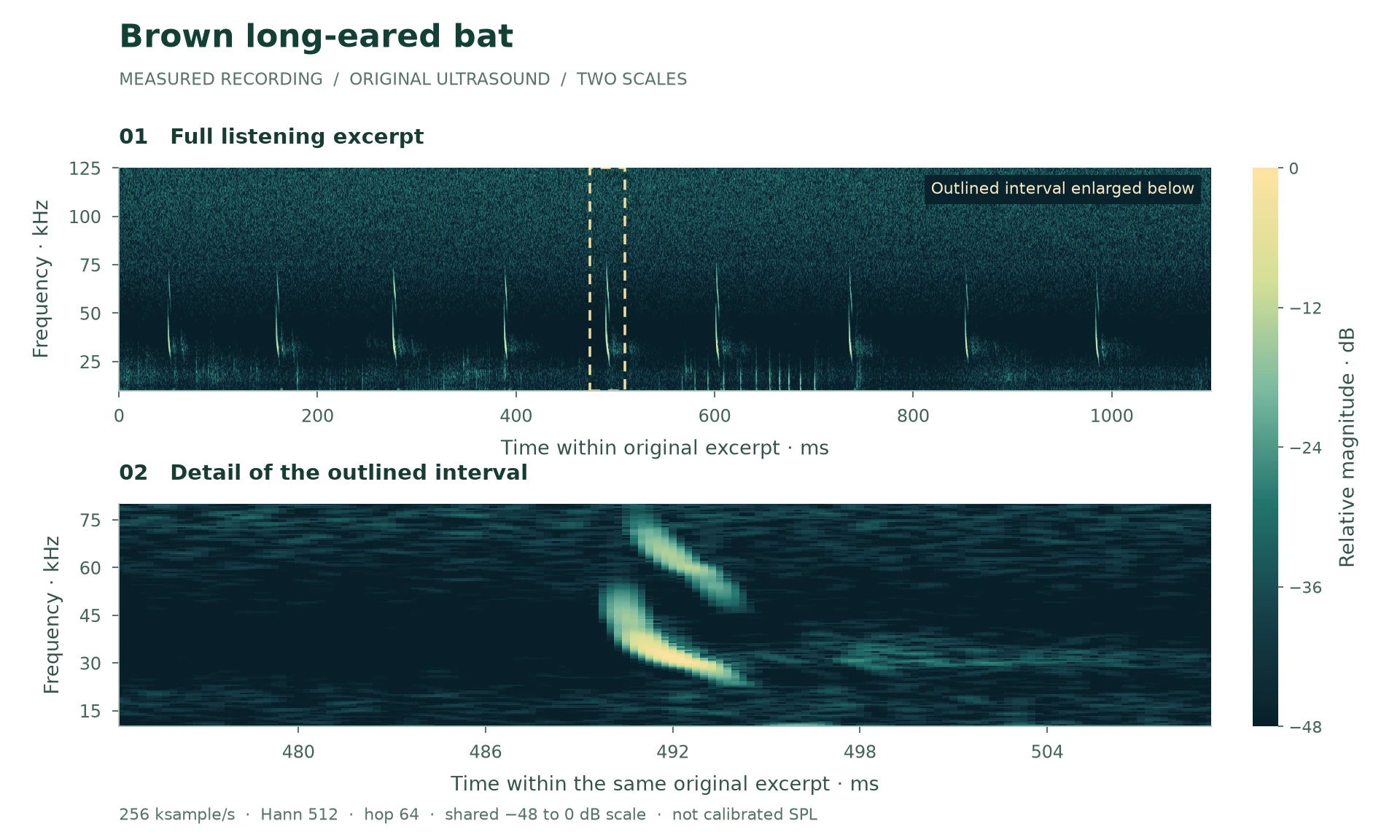
Plecotus auritus
10× slower · 11.0 seconds
Broad downward sweeps and faint calls illustrate why long-eared bats can be difficult to detect. This community-labelled example does not provide a reliable sound-only distinction from grey long-eared bat.
Recording credit: (c) Uploads from the Somerset Bat Groups events and members, some rights reserved (CC BY)
(c) Uploads from the Somerset Bat Groups events and members, some rights reserved (CC BY) · CC BY 4.0. Recorded in United Kingdom; this is not an ACP project recording. iNaturalist research; community identification, not independent ACP confirmation.
Original 256 ksample/s; channel 1. Excerpt 1.553–2.653 seconds. Playback is 10× slower, with frequency divided by ten and duration multiplied by ten. Gain was normalised, then resampled to 32 kHz for MP3. No denoising was applied.
The spectrogram uses original samples, a 512-sample Hann window and a 64-sample hop. Levels are relative to the strongest plotted component, not calibrated dB SPL. Original files and processing records are retained.
The lower plot enlarges 474.2–509.2 ms within this excerpt. It selects a high-energy interval within the documented analysis band. This is a visual teaching detail, not an independently verified species identification. Both plots use the same −48 to 0 dB reference.
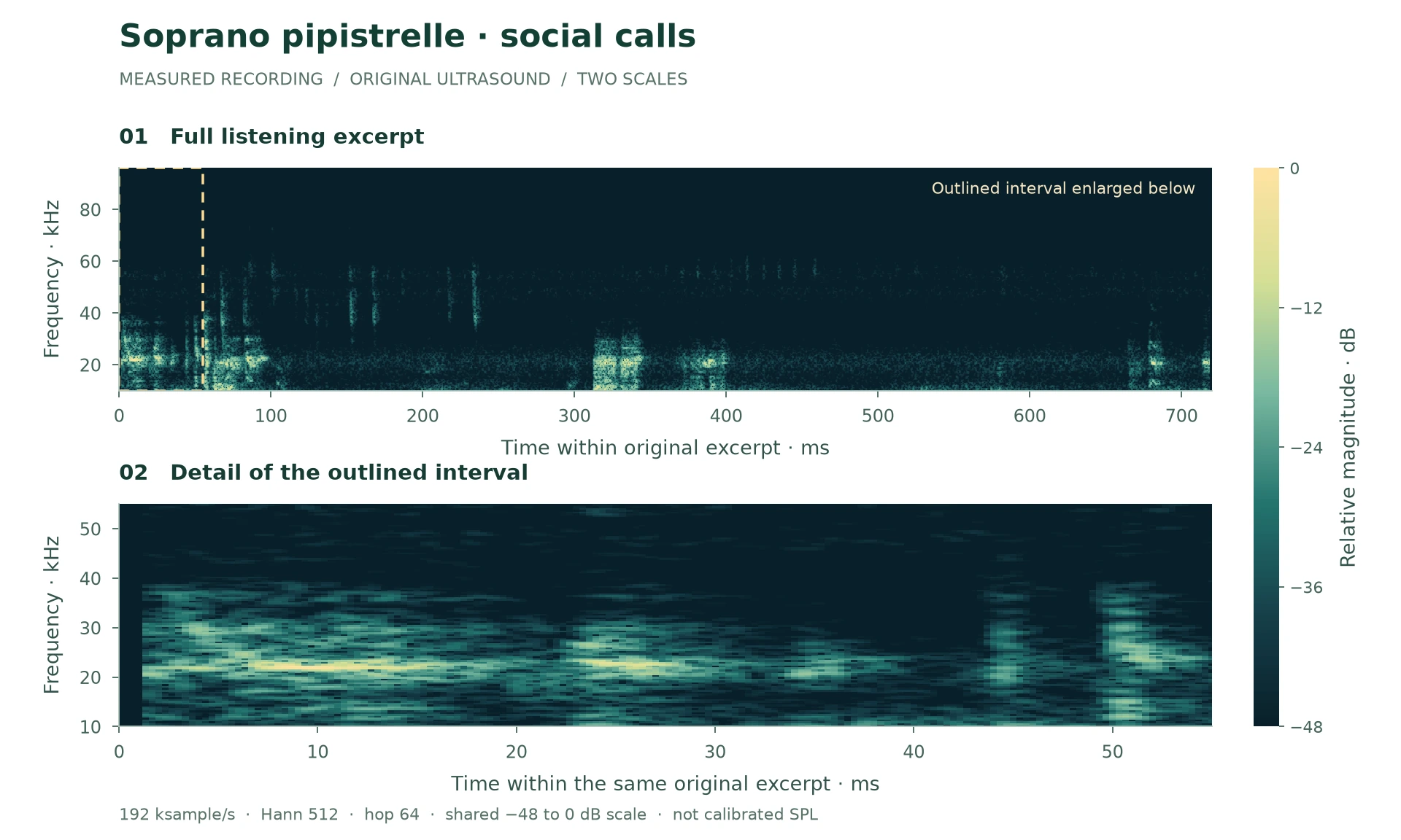
Pipistrellus pygmaeus
10× slower · 7.2 seconds
Listen for the varied, clustered sounds and compare their structure with the regular search-call examples. The recordist reports bats at a roost, and the repository labels these as soprano pipistrelle social calls. We have not independently confirmed the species or the function of each syllable.
Recording credit: Christian Kahle, XC1031662 (2025)
Christian Kahle, XC1031662 (2025) · CC0 1.0. Recorded in Germany; this is not an ACP project recording. Repository and community label: soprano pipistrelle social calls; species not independently confirmed by ACP.
Original 192 ksample/s; channel 1. Excerpt 0.050–0.770 seconds. Playback is 10× slower, with frequency divided by ten and duration multiplied by ten. Gain was normalised, then resampled to 32 kHz for MP3. No denoising was applied.
The spectrogram uses original samples, a 512-sample Hann window and a 64-sample hop. Levels are relative to the strongest plotted component, not calibrated dB SPL. Original files and processing records are retained.
The lower plot enlarges 0.0–55.0 ms within this excerpt. It selects a high-energy interval within the documented analysis band. This is a visual teaching detail, not an independently verified species identification. Both plots use the same −48 to 0 dB reference.
A complete sequence may contain several species or call types. The original file, channel and excerpt times are documented with each example. Detector or microphone details are not invented where the source record does not provide them. Research-dataset methods are linked alongside community record credits.
Disturbance, masking and detectability
A noisy recording and a disturbed bat are two different findings. Noise may obscure a microphone’s detection without changing bat activity. Alternatively, bats may alter behaviour, avoid an area or change vocal output. Therefore, a study must distinguish between these causes.
Direct masking depends on the signal and noise reaching the receiver within relevant auditory filters and time windows. Broad frequency overlap is useful context, but it is not enough to calculate a bat’s hearing threshold. However, noise outside an echolocation band can also distract an animal or affect its use of prey-generated sounds.
Road, rail and aircraft noise vary by event and spectrum. Construction and industrial sources may be impulsive, tonal or broadband. Wind, rain, insects and moving water also influence recordings. An audible description such as “quiet” does not prove a low ultrasonic noise floor.
A study of wild Daubenton’s bats used controlled light and ultrasonic broadband noise exposures with passive acoustic monitoring at different distances. Reported activity reductions close to the sources differed from responses farther away.
This supports concern about sensory disturbance under the tested conditions. However, it does not supply a universal setback, a safe lux threshold, or a dB(A) limit for every bat species and site.
For a development assessment, describe source operating times, spectra, propagation paths and the ecological functions nearby. Therefore, combine acoustic evidence with habitat, lighting and behavioural context. Our bats and lighting guide addresses the interacting lighting question.
Evidence: Caspersen et al. (2026), light and ultrasonic noise effects on Daubenton’s bats · Jespersen et al. (2022), UAV-borne microphone array.
Laboratory 07 · signal and background
This teaching tool places a schematic bat-call spectrum beside different example noise shapes. Change their relative levels to see why comparing only a peak frequency is not enough.
Signal-to-noise ratio in dB, using powers measured over the same frequency band and time interval.
If band-limited signal power is ten times noise power, SNR is 10 dB. If they are equal, SNR is 0 dB. However, these ratios do not define a universal detector threshold: algorithms, call structure and false-positive tolerance affect detection.
The plotted curves are shapes chosen for teaching, not measurements of a real road, factory or rainfall event. The displayed SNR comes from the stated same-band level inputs; it is not inferred from the cartoon spectra.
For a valid comparison, signal and noise inputs must refer to the same analysis band, interval and reference. Comparing a narrowband pulse level with a whole-recording broadband noise number can give a misleading ratio.
Choose the low-frequency background, then the narrowband example. The shapes show where energy lies; the numeric SNR remains a separate controlled example. In contrast, a real masking model would need the receiving animal’s relevant auditory filters and detection behaviour.
Relative common-reference levels, not dB SPL. Conceptual spectra only; no biological masking, ecological harm or detection probability is calculated.
© 2026 ACP Consultants Ltd. · Original educational diagramEvidence: Caspersen et al. (2026), light and ultrasonic noise effects on Daubenton’s bats · Goerlitz (2018), weather, attenuation and monitoring.
Uncertainty is part of the result
Automated software can sort large collections and identify likely candidates for review. In practice, performance depends on the species represented, recording conditions, version and decision threshold. However, one model’s confidence score is not automatically a calibrated probability of the species being present.
A 2026 systematic review screened literature published from 1990 to 2022. Its publication date is recent, but its underlying evidence does not include every current software release. It found large differences and called for checks, rather than accepting automated outputs on their own.
Perks and colleagues’ 2026 comparison used recordings from Anabat and AudioMoth at four Worcestershire sites. The study tested different classifier combinations on those detector datasets. However, agreement between tools is useful to investigate, but it is not the same as independently verified identification accuracy.
A rare target can produce many false positives even when a classifier’s headline performance looks good. Review plausible alternative species, microphone artefacts, overlapping calls and geographical context. If the evidence cannot separate species, retain a group-level result.
Suppose 10 of 1,000 clips truly contain a target species. An example classifier detects 90% of those clips and incorrectly flags 5% of the other 990.
Expected true positives = 9. Expected false positives = 49.5. Positive predictive value is 9/(9 + 49.5), or 15.4%. The fractional count is an expectation across repeated samples.
This is a worked example, not a performance claim for any product. Instead, it explains why sensitivity, false-positive rate and prevalence must be assessed together.
Precision = TP/(TP + FP); recall = TP/(TP + FN). Specificity = TN/(TN + FP). Therefore, report the class definitions, sample unit and denominators. A “clip”, “pass” and “individual bat” are different units.
Do not randomly split near-identical calls from the same pass into training and test sets and then claim that the model works on new, independent data. Instead, separate sites, dates, individuals or recording sessions where the question requires it. Keep a held-out test set and report per-species results, not only overall accuracy.
If an example binomial estimate gives 90 successes in 100 independent trials, the standard error is about √[0.9×0.1/100] = 0.03. Independence and a defensible reference label matter; repeated calls from one bat do not automatically provide 100 independent tests.
Evidence: Pino-Aedo & Muñoz-Sáez (2026), systematic review of echolocation analysis · Perks, O’Connell & Goodenough (2026), classifier comparisons.
An audit trail, not just an image
Retain the source WAV, sample rate, channels, detector settings and file checksum. Keep precise roost locations in protected project records. Public learning examples do not need confidential coordinates.
Log channel selection, crop boundaries, DC removal, filters, gain, resampling and display settings. Keep scientific measurements on original-rate samples. Then create separate compressed, slowed listening copies.
Store the measured pulses, alternative species, confidence and reviewer. Record why a call was excluded. A reproducible figure is useful evidence; a visually tidy trace alone is not a validated identification.
This example needs NumPy, SciPy, SoundFile and Matplotlib. Use a lawfully obtained original WAV, not the slowed MP3 player. Set channel and crop from the provenance notes. Also record package versions with the output.
import numpy as np
import soundfile as sf
from scipy.signal import spectrogram
import matplotlib.pyplot as plt

x, fs = sf.read("original.wav", always_2d=True)
channel = 0                  # zero-based channel index
start, duration = 5.55, 0.90 # seconds: research soprano example
y = x[round(start*fs):round((start+duration)*fs), channel]
y = y - y.mean()            # record this DC-removal step
f, t, z = spectrogram(y, fs, window="hann",
    nperseg=512, noverlap=448, detrend=False,
    scaling="spectrum", mode="magnitude")
reference = max(z.max(), 1e-15)
db = 20*np.log10(np.maximum(z, 1e-15)/reference)
plt.pcolormesh(t*1000, f/1000, db, shading="auto",
               vmin=-48, vmax=0)
plt.ylim(10, min(125, fs/2000))
plt.xlabel("Original time (ms)")
plt.ylabel("Original frequency (kHz)")
plt.colorbar(label="Relative magnitude (dB)")
plt.show()
The 64-sample hop follows from 512 − 448. This produces a relative display. However, it does not estimate calibrated SPL or automatically identify the species. Longer R/Python workflows can also add measured-call selection, quality flags and independent validation.
Evidence: SciPy, ShortTimeFFT documentation · Jespersen et al. (2022), UAV-borne microphone array.
Connect measurements to decisions
A detector samples the acoustic space around its microphone. Quiet calls, off-axis flight, blocked paths and equipment response affect what is recorded. However, more files do not necessarily mean more bats; repeat passes can come from the same bat.
First, design survey effort around a question. Static detectors can describe activity at selected positions across nights. Walked surveys also add observation and spatial context. Emergence work needs evidence tied to a structure or access feature, often combining direct observation and night-vision recording.
BCT’s fourth-edition guidance remains the current edition listed on its guidance page, with a downloadable text amended in March 2024. Its scope includes auto-identification and data science. However, guidance informs professional judgement; this learning page does not replace its survey design requirements.
In an ACP final emergence report previously checked for our case-study library, two dusk visits combined attended observations with reviewed infrared footage. Bat activity occurred nearby, while the report concluded likely absence for the assessed building.
The key point is the difference between a bat passing a detector and evidence of emergence from a building. The earlier PRA was prepared by another consultancy. This example does not claim planning approval, completed works or measured mitigation success.
The scientific audio examples use attributed external sources. The ACP report example is separate evidence; it is not the provenance of those recordings.
For a project, use bat activity surveys to understand the service scope, or send ACP the site details and the decision you need to make. We can discuss what evidence is proportionate, including design options that avoid impacts where feasible.
Evidence: BCT, Bat Surveys for Professional Ecologists, fourth edition · Natural England, bats and planning decisions.
From discovery to modern methods
The physical account of sound links pressure, density and particle motion. Mathematical models make testable predictions about speed, wavelength, interference and reflection. Modern recordings add calibrated sensors and digital analysis to that foundation.
Griffin’s retrospective describes the experimental identification of ultrasonic bat signals with Robert Galambos and the development of echolocation research. His 1958 book Listening in the Dark helped frame a wider comparative study of animal orientation.
Modern arrays can estimate positions and examine directionality while recording behaviour. Jespersen and colleagues tested a suspended array beneath a UAV, explicitly measuring platform noise. Their design therefore shows why the observer’s equipment is part of the experiment.
Scientific progress is not a sequence of ever-more-certain labels. Instead, better instruments also reveal variation and limits. Published work on changing call sequences, atmospheric effects and classifier disagreement makes those limits part of good practice.
Evidence: Griffin (1987), retrospective on Listening in the Dark · Jespersen et al. (2022), UAV-borne microphone array · Goerlitz (2018), weather, attenuation and monitoring.
Quick answers · open only what you need
A bat emits sound and processes returning echoes. Delay provides information about distance; direction, spectrum and changes between echoes add information about the scene. The animal adapts calls and flight rather than simply emitting an unchanging tone.
Most British bat echolocation is ultrasonic. Some lower-frequency components and social sounds may be audible to some people. The players here use tenfold slowed copies, not unmodified ultrasound.
The sound travels to the target and back. Multiplying delay by sound speed gives the round-trip path; half of that path is the target distance in the simple stationary model.
No. Frequency is one clue. Call shape, sequence, behaviour, equipment, geography and alternative species must also be considered. A single number is not an identification key.
Not automatically. Its colour scale may show relative magnitude, relative power or another convention. Physical SPL requires a calibrated chain and a defined reference and bandwidth.
An ordinary phone microphone and audio sample rate do not directly capture most bat ultrasound. An ultrasonic accessory supplies suitable sensing hardware; the phone provides recording and display functions.
Not necessarily. One bat can make repeated passes, and detection varies with calls, equipment and conditions. Activity measures need defined units and cannot automatically be converted into an individual count.
A longer window uses a longer time interval and gives smaller frequency-bin spacing. A shorter window follows rapid changes better. Window shape, signal duration and noise also influence the result.
No. It is one part of the context. A defensible conclusion needs exposure, auditory or behavioural evidence, species and activity context, and appropriate controls.
No. The sound examples use licensed external recordings. Every example identifies the creator or source, links the original record and states the licence and processing. The separate ACP project example is report-based.
No. They are educational models. Detection distance also depends on source level, directivity, atmosphere, habitat, equipment, noise and the detection criterion.
Keep the original WAV, device and microphone details, settings, effort, weather, placement and timestamps. Preserve processing history, measured call selections, uncertainty and reviewer decisions.
Books, editions and actual access
The open university chapters and full research papers support the explanations above. These established books offer further study. Access is stated explicitly: a publisher description or sample is not a claim that the full textbook has been consulted.
Kinsler, Frey, Coppens & Sanders (2000)
Wiley; ISBN 9780471847892
Publisher or authorised sample
Publisher contents and bibliographic record checked; full book not reviewed.
Rossing, Moore & Wheeler (2014 international edition)
Pearson; ISBN 9781292039572
Publisher or authorised sample
Available publisher sample reviewed; not the complete book.
Pierce (2019)
Springer; DOI 10.1007/978-3-030-11214-1
Publisher or authorised sample
Publisher record and contents checked; full text not reviewed.
Altringham (2011)
Oxford University Press; ISBN 9780199207114
Publisher or authorised sample
Publisher record and abstract checked; full book not reviewed.
Fenton & Simmons (2015)
University of Chicago Press
Publisher or authorised sample
Publisher description checked; full book not reviewed.
Russ, editor (2021)
Pelagic Publishing; ISBN 9781784272258
Publisher or authorised sample
Specialist reference and companion library; publisher description, not full book, reviewed.
Traceable evidence
Research refreshed 14 November 2026. References are linked beside the claims they support. The following register separates open explanatory chapters, full papers, guidance and methodological documentation. Recording creators and licences appear with each player. Original teaching diagrams are ACP artwork; third-party audio and derived spectrogram examples are attributed to their sources.