Environmental consultancy for planning & development0330 236 7329hello@acp-consultants.com

ACP learning resource · R & Python

Bat survey data analysis: practical R and Python

Turn recordings and survey records into results you can explain, check and reproduce.

Work through a real attributed recording, an invented activity dataset and clear examples of statistical uncertainty. Download the code, inspect the calculations and adapt the workflow to your own question.

Each lesson has a Python and an R implementation. The supplied examples have been run in both languages, with matching numeric outputs.

Start with the question, then choose the measurement

For ecologists, students and curious analysts

You can use these lessons to learn how an acoustic analysis is assembled. They also provide a transparent starting point for discussing a dataset with a colleague or supervisor.

To begin, some familiarity with files, tables and running a script will help. You do not need paid acoustic software for the supplied examples. First, choose one language. Then compare the results if you want to explore how the code works.

For the underlying sound physics, read our bat echolocation and acoustics guide. For British species and identification limits, use the British bats reference.

Keep the ecological meaning in view

For example, a recorder samples sound at a particular place and time. Your analysis should say what that sample represents, what was missed and which comparisons the design supports.

  • A pulse, a sound file, a pass and an individual bat are different units.
  • A reviewed zero needs valid recording effort. A failed recording is missing evidence.
  • A numerical result does not decide whether a planning survey is sufficient.

Our survey guidelines and methods guide explains the wider survey context.

Download the scripts, data and expected results

ACP BAT DATA TOOLKIT · V1.0

Run all three lessons in either language

The ZIP contains six lesson entry scripts, shared functions, a source recording, synthetic survey data, a data dictionary, licences and numeric reference outputs. It also includes a checker for the unchanged examples.

No account or paid analysis package needed.

Python quick start

Install Python, unzip the toolkit and open a terminal in its folder. The Windows commands below use an isolated environment without changing activation settings.

python -m venv .venv
.venv\Scripts\python.exe -m pip install -r requirements.txt
.venv\Scripts\python.exe python/01_acoustics.py
.venv\Scripts\python.exe python/02_activity.py
.venv\Scripts\python.exe python/03_uncertainty.py

On macOS or Linux, use .venv/bin/python as the interpreter. Those platforms have not been separately tested. The README includes input and output options.

R quick start

Install R from CRAN and open a terminal in the unzipped folder. The examples use base R, so no extra R packages are required.

Rscript --vanilla R/01_acoustics.R
Rscript --vanilla R/02_activity.R
Rscript --vanilla R/03_uncertainty.R

Use the full path to Rscript if it is not on your PATH. These are terminal commands; they are not intended for the R console.

Outputs go into separate outputs/python and outputs/R folders. Re-running a lesson replaces its output files. Choose a new --out folder when comparing settings.

What is inside the download
IncludedPurposeReuse terms
Python and R scriptsAcoustic measurements, effort summaries and uncertainty examples. Shared functions keep each calculation inspectable.Original ACP code: MIT licence.
Original-rate recording and listening copyA real 1.1-second excerpt, plus the same samples played 10× more slowly.External recording: CC BY 4.0, with creator, source and modifications retained.
Synthetic CSV and data dictionary24 planned site-nights across eight invented sites, with zeros, downtime and an exclusion.Invented ACP teaching data: CC0. Do not describe it as a real survey.
Expected results and checksCSV outputs, a regression checker and the actual test record.Checks verify the supplied exercise, not the validity of a different study.

FREE BROWSER TOOLS · NO INSTALLATION

Explore your data before running a model

Start with the worked examples, then open a copy of your own records. Your survey inputs stay on your device. Save the exports before closing the browser.

Check recording effort and data quality

Map your columns, inspect missing or failed nights and compare reviewed activity using the valid recording effort. Keep the audit, assumptions and source records with any exported chart.

CSV · up to 5 MB · 20,000 rows

Measure an original-rate recording

Choose a channel and time window, then inspect its waveform, spectrogram and mean spectrum. Export the settings, source credit and a labelled measurement log.

WAV · up to 64 MB · two-second analysis windows

Review aids with clear limits. These tools support data review. They do not identify species, count individual bats, establish absence or replace professional judgement. Read the instructions, examples and limitations before interpreting a result.

Then use the R or Python scripts below for a reproducible workflow that matches your question and study design.

Build a dataset that preserves the field evidence

Keep an effort table as well as detections

Begin with every planned sampling unit. Then join the observations to that schedule. Starting only with files containing bats can make valid zero nights disappear.

Here, a row means one site-night for one consistently reviewed taxon or acoustic group. The counts have already been checked and aggregated. The scripts do not infer a pass from a filename or classify an unknown recording.

In a real project, retain the raw event table too. It should connect each accepted sequence to its original recording, review decision and deployment. Resolve duplicate or overlapping files using a written rule.

Write down the decisions before comparing sites

  • Define the question, target taxon/group and sampling unit.
  • Specify the recording schedule, usable intervals and exclusion rules.
  • Record detector, microphone, settings, location and clock/time-zone information.
  • Keep classifier output separate from reviewed labels and unresolved records.
  • Preserve original files and record any cropping, conversion or filtering.

If sites were selected beside likely flight routes, say so. A targeted sample does not automatically represent a whole landscape.

The supplied CSV: essential fields, units and rules
FieldMeaningExample rule
site_id + nightA unique sampling-unit key.S03, 2026-07-02. The date labels the night’s start; handle overnight times before aggregation.
planned_hoursThe intended sampling window.8 hours, including time subsequently lost to recorder failure.
valid_hoursUsable operating time matched to the accepted count.6 valid hours out of 8 planned hours. Triggered-file duration is not recording effort.
reviewed_passesAccepted passes under one declared definition.0 is a reviewed zero. A blank is missing, and must accompany zero recording effort.
status + noteA separate analysis decision and explanation.included, excluded or not_recorded. Never silently delete an inconvenient result.

A partial night needs an honest denominator

If a detector worked for six usable hours, count only the accepted passes within those same intervals. However, dividing a whole-night count by six hours would inflate the rate.

Likewise, a triggered recorder can remain available for hours while saving short clips. Adding the clip durations measures stored sound, not the time during which the detector could record. Scheduled sleep needs separate treatment.

Standardisation does not make equipment identical

The 2025 UK study by Perks and colleagues compared commercial and open-source configurations in several habitats. Its methods included different recording schedules and detector deployment choices.

That matters when interpreting a rate. Document hardware, firmware, microphone condition, trigger rules and sleep schedules. Therefore, a simple per-hour adjustment does not remove every difference in detectability.

Lesson 1: analyse a real bat recording

Use the original-rate WAV for measurements

The supplied excerpt contains 281,600 samples at 256,000 samples per second. It lasts exactly 1.1 seconds. However, its source community identifies common pipistrelle, Pipistrellus pipistrellus; ACP has not independently confirmed that identification.

The scripts read mono 16-bit PCM WAV files. They retain the original sampling rate and calculate a digital waveform, mean spectrum and spectrogram. They also reject an unsupported channel/bit-depth format and an analysis band above Nyquist.

The cropped source has not been denoised or normalised. For traceability, its provenance file records the original hash, crop start, sample count and licence.

Listen, then inspect the figure

This player uses the same samples at one tenth of the original sample rate. As a result, the 11-second listening version makes the sequence audible. It also lowers every frequency by a factor of ten.

Analyse reference_excerpt.wav, not the listening copy. Changing a header for playback is not a new ultrasonic recording.

Recording © Uploads from the Somerset Bat Groups events and members. Original source · CC BY 4.0. Cropped and slowed for this demonstration.

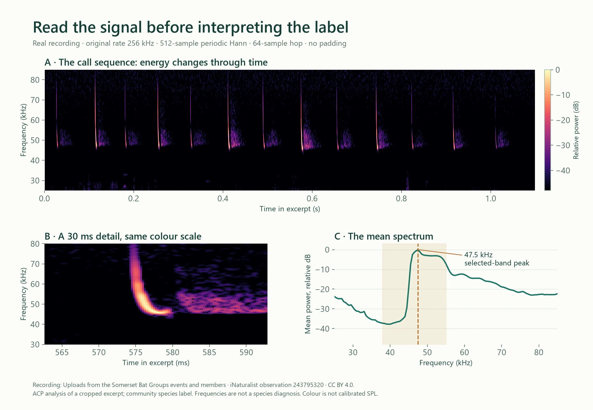
Spectrogram of an attributed real common-pipistrelle recording, a 30 millisecond detail, and a mean spectrum with a 47.5 kilohertz peak in the selected band.
Read A, then B, then C. The upper panel shows the sequence. The lower-left panel enlarges 30 ms around the strongest frame; it is not an automatically segmented call. The lower-right panel averages window power. Its shaded band marks the selected 38–55 kHz search range. Open the full-size figure ↗
Recording © Uploads from the Somerset Bat Groups events and members · source observation · CC BY 4.0. Cropped excerpt; analysis by ACP. ACP does not own the recording.

What the script actually calculates

A spectrogram applies a short Fourier transform repeatedly along the signal. Specifically, this example uses a periodic Hann window and only complete frames. Also, it performs no padding, filtering or detrending.

window[j] = 0.5 - 0.5 × cos(2πj / N)
power = |FFT(window × samples)|²
relative dB = 10 × log10(power / maximum power)

The mean spectrum averages power across frames before converting it to relative decibels. The reported peak is the largest FFT bin inside the chosen band. However, it is not automatically the call’s end frequency or characteristic frequency.

  • acoustic_metrics.csv records the settings and measured values.
  • mean_spectrum.csv preserves every frequency bin.
  • acoustics.png shows the waveform and spectrogram.

Read the numerical output

Expected values for the supplied excerpt
Setting or resultDefault value
Sampling rate256 kHz; Nyquist frequency 128 kHz
FFT size and window512 samples; 2 ms
Hop64 samples; 0.25 ms
Frequency-bin spacing500 Hz
Complete frames4,393
Selected-band mean-spectrum peak47.5 kHz

Change one parameter and compare

A 2,048-sample window gives 125 Hz bin spacing at this sample rate, but spans 8 ms. However, that longer window can smear rapid frequency changes. Smaller bin spacing is not automatically a better description of a short call.

python python/01_acoustics.py --fft-size 2048 --hop 256 --out outputs/long-window

Rscript --vanilla R/01_acoustics.R --fft-size 2048 --hop 256 --out outputs/R-long-window

Use your virtual-environment Python interpreter. Compare the figures and CSVs; keep both output folders. Reducing the hop adds overlapping frames, not independent acoustic events.

Three limits to report with the figure

  • Frequency is not an identity. A peak depends on the sequence, recording conditions and selected band. Do not turn 47.5 kHz into a species rule.
  • Colour is not sound pressure level. The spectrogram is relative to its own maximum. Comparing normalised colours cannot show which bat was louder.
  • No rail samples does not prove no clipping. The PCM-rail check is a useful flag, but distortion can arise earlier in the recording chain.

The acoustics guide explains call structure, recording methods and identification in more detail.

Lesson 2: calculate bat activity per valid recording hour

Run the effort-aware summary

This lesson uses invented, already-reviewed pass counts. It does not use the real WAV to manufacture a survey dataset. Each included count covers the same usable time interval as its denominator.

python python/02_activity.py
Rscript --vanilla R/02_activity.R

The scripts reject duplicate site-nights, negative effort, fractional pass counts and missing counts on included nights. They also preserve exclusions and failed recordings in a separate audit table.

For your own file, supply --input "your-summary.csv" and a fresh --out directory. Read the data dictionary first.

Check the audit before the headline number

  • 24 planned site-nights.
  • 21 included site-nights with reviewed counts.
  • 2 nights with no usable recording; counts stay blank.
  • 1 night excluded under the invented protocol.
  • 2 included nights with genuine zero passes.

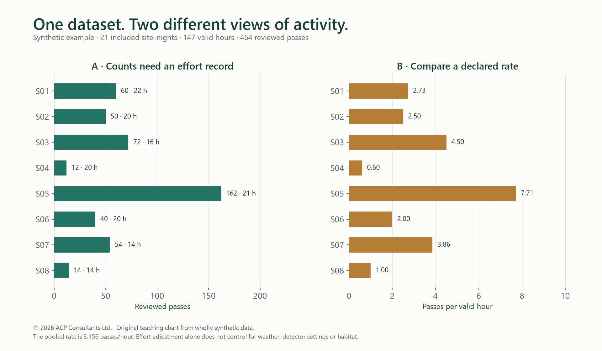
The accepted data contain 464 passes in 147 valid hours. The programme produces a site summary, a night audit, a figure and machine-readable metrics.

Open night_audit.csv first. Check that every planned row remains visible and that blank rates have an explained status. Then reconcile the accepted totals with your reviewed source records.

Eight invented sites shown as pass counts with valid hours and as passes per valid hour, demonstrating why raw counts need an effort denominator.
Counts and rates answer different descriptive questions. In the left panel, each label includes valid hours. The right panel divides each site’s accepted total by its own valid hours. These are invented teaching values, not ACP project results. Open the full-size figure ↗
ACP ConsultantsOriginal educational chart
© 2026 ACP Consultants Ltd.

The pooled rate weights recorded effort

pooled rate = sum(reviewed passes) / sum(valid hours)
            = 464 / 147
            = 3.156462585 passes per valid hour

This describes the accepted recording effort pooled across the example. Consequently, a site with more valid hours contributes more to that pooled result.

It is useful when the target is activity per unit of combined effort. However, it does not give every site equal influence. State which population of observations your summary represents.

The equal-site mean gives each site one vote

site rate = site passes / site valid hours
equal-site mean = mean(site rates)
                = 3.112337662 passes per valid hour

In contrast, this first calculates eight site rates, then averages them. As a result, a site with more hours no longer receives more weight in that final mean.

The two answers differ because they estimate different summaries. Neither is universally preferable. Choose the estimand—the quantity you intend to describe—before drawing a conclusion.

Do not count a pass as an individual bat

A single bat can return to the microphone repeatedly. Conversely, bats may pass outside its useful detection volume. Grouping pulses into a sequence does not identify individuals.

Roemer and colleagues’ 2025 perspective discusses the unresolved relationship between acoustic activity and population measures. That is why this tutorial reports passes and effort, without converting them into a number of bats.

Compare like with like

Keep the taxonomic grouping and pass definition consistent. Otherwise, pooling species with different acoustic detectability can obscure the ecological question.

For a site comparison, also examine season, weather, habitat, microphone position and configuration. If these differ systematically, a rate table alone cannot separate their effects. Our bat activity surveys guide connects this analytical issue to survey design.

Lesson 3: show uncertainty without inventing certainty

Resample the units that match the question

Here, the target is the equal-site mean. The exercise assumes eight independent, exchangeable sites. Each bootstrap replicate samples eight site rates with replacement and takes their mean.

In contrast, the nights remain inside their original site summary. Resampling every sound pulse or file as an independent site would create an artificial impression of replication.

python python/03_uncertainty.py --replicates 2000 --seed 20261116
Rscript --vanilla R/03_uncertainty.R --replicates 2000 --seed 20261116

Read this interval as a teaching example

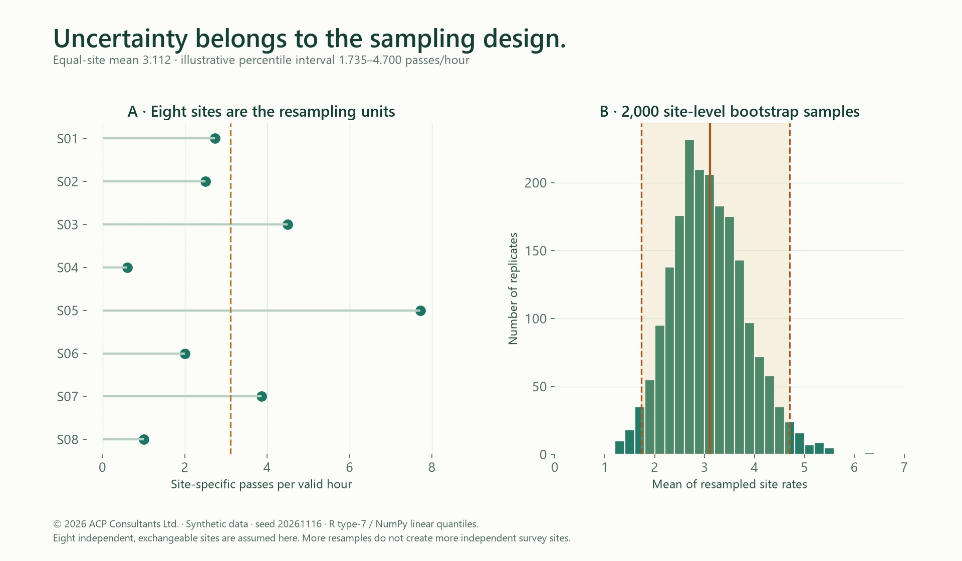
The 2,000 resamples give an equal-site mean of 3.112 passes per valid hour. Their 2.5th and 97.5th percentiles are 1.735 and 4.700.

The interval illustrates one method on a very small invented dataset. However, it does not include species-identification error, imperfect detection or biased site selection. Therefore, it is not a population estimate or a measure of habitat importance.

With real spatial clusters or repeat survey rounds, choose a resampling or model structure that reflects those dependencies.

Site rate dot plot and distribution of 2000 bootstrap site means, with mean 3.112 and a teaching percentile interval from 1.735 to 4.700 passes per hour.
The left panel shows the eight rates being resampled. The right panel shows the resulting means. The solid line marks the equal-site mean; dashed lines mark the percentile endpoints. Moreover, more bootstrap replicates refine the calculation but do not create more independent sites. Open the full-size figure ↗
ACP ConsultantsOriginal educational chart
© 2026 ACP Consultants Ltd.

Why the R and Python results match

Matching seed numbers alone do not guarantee matching random samples across languages. This is because R and NumPy have different default random generators.

For this exercise, both scripts implement the same documented Park–Miller sequence. They map it to the same site indices and use the same quantile definition: R type 7 and NumPy’s linear method.

The checks compare all 2,000 bootstrap means, not just the rounded endpoints. This deliberate choice makes the example easy to audit; it is not a claim that one random generator suits every statistical task.

Ask what the interval leaves out

  • Were sites selected independently and from the population you want to describe?
  • Do nearby detectors share the same bats or weather effects?
  • Were review errors or rejected calls distributed unevenly?
  • Does each site have enough comparable seasonal coverage?
  • Would a different legitimate metric or quality rule change the conclusion?

Therefore, an apparently narrow interval can still describe a biased or unsuitable dataset.

Explain non-detection with the condition still attached

The calculation is conditional on presence

Suppose the chance of a detection on each independent visit is a known constant p. If presence and availability are coherent over the sampling period, the chance of at least one detection is:

P(at least one detection | present) = 1 − (1 − p)ⁿ

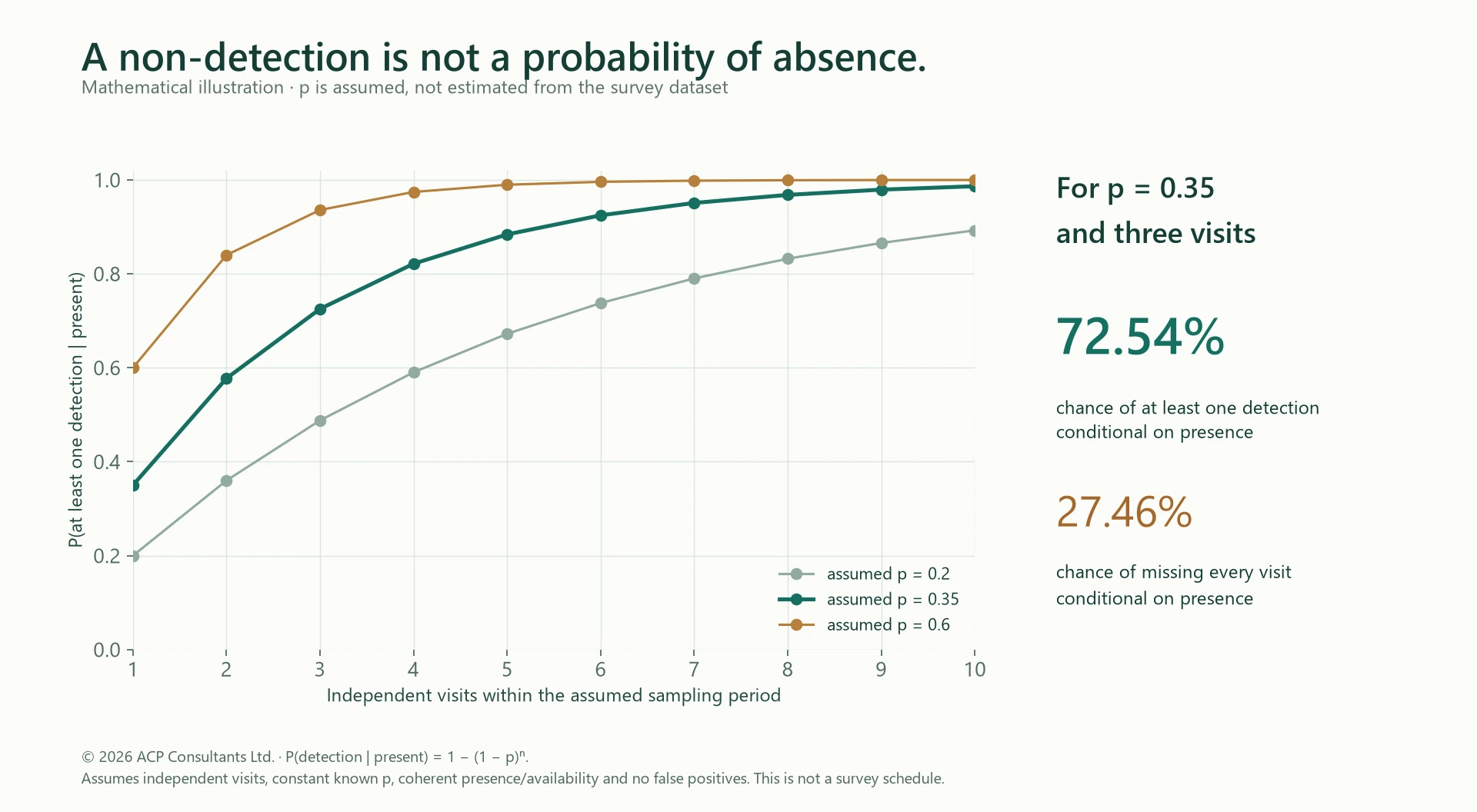
The vertical bar means “given”. With the invented value p = 0.35 and three visits, the result is 72.5375%. The chance of missing every visit, despite presence, is 27.4625%.

For this example, the scripts use --detection-p 0.35. This value is an assumption. It is not estimated from the activity dataset.

Do not reverse the probability

A 27.46% chance of missing a present species is not a 27.46% chance that bats are absent. In other words, those are different conditional statements.

To estimate occupancy from repeated observations, you need a suitable observation model and a study design that supports it. For example, availability, varying detection and false positives can change the analysis.

The curve also does not prescribe a number of survey visits. Apply current professional guidance and project-specific judgement to the actual survey question.

Conditional detection curves for assumed per-visit probabilities of 0.2, 0.35 and 0.6. At p 0.35, three visits give 72.54 percent detection if present, not a probability of absence.
These curves compare three invented per-visit detection probabilities. They assume independent visits, constant known detection probability and no false positives. They do not calculate the probability of absence after a survey. Open the full-size figure ↗
ACP ConsultantsOriginal educational chart
© 2026 ACP Consultants Ltd.

Build a detection history deliberately

For an occupancy analysis, a repeated-survey table typically records accepted detection, valid non-detection or missing survey. A valid zero needs an observation process capable of detecting the target under the study protocol.

Converting every classifier label to a 1 can introduce false positives. Similarly, converting equipment failures to 0 can introduce false negatives. Preserve review uncertainty so an appropriate model can use it.

False-positive models need more information

Clement and colleagues’ 2014 study explicitly modelled uncertain acoustic detections alongside a second observation method. It illustrates why identification error is part of the model design.

However, that US study is not a source of ready-made UK error rates. Our download demonstrates the conditional arithmetic only. It does not fit an occupancy model or claim that the example meets its assumptions.

Choose a statistical model that matches the evidence

Once the descriptive checks are complete, a more advanced question may need a model. Start with the response, sampling unit and observation process. Then decide how to represent effort, dependence and uncertainty.

Analysis routes: starting points for study design, not automatic prescriptions
QuestionPossible approachChecks before relying on it
How does recorded activity vary with a measured factor?A count model may include log(valid effort) as an offset. A negative binomial model may suit overdispersion; a mixed model may represent repeated sites.Check the count definition, unequal observation processes, dispersion, residuals, dependence, influential units and whether the effort relationship is defensible.
Where is a target species likely to occur?A repeated-survey occupancy model separates occurrence from detection under explicit assumptions.Assess closure/availability, repeated sampling, covariates, species review and false-positive handling. A site history is not the same as a pass total.
Did a measure change activity through time?A planned before–after/control–impact design or suitable hierarchical time model may help.Check comparable effort and season, control sites, timing, intervention effects and confounding. A simple before/after difference does not establish causation.
How well does an automated classifier perform?Use independently labelled validation data, an explicit error matrix and sensitivity analyses.Separate training and validation by the relevant site/recording unit. Avoid leakage between related calls. Report performance for the intended domain and taxonomic group.

An effort offset has a specific meaning

In a log-link count model, a common formulation is log(E[count]) = predictors + log(effort). The offset fixes the effort coefficient at one. In other words, this encodes proportional exposure, conditional on the model.

It does not make two recording protocols equivalent. Also, a higher fitted count need not mean more individual bats. The response still describes the recorded and reviewed acoustic metric.

The download does not fit this model. That prevents a toy result from appearing to validate a real ecological inference.

Review the whole analysis pipeline

A 2026 paper by Isenhour and colleagues compares data-handling techniques for modelling acoustic activity. We reviewed its abstract and bibliographic record; the full text was not retrieved.

It is a useful current reading lead for analysis planning. We have not copied its methods or numerical findings into the toolkit. For a real study, test reasonable processing decisions and record their effect on the result.

Adapt the code and leave a trail another analyst can follow

A practical reuse checklist

  • Copy the original files into a read-only source folder and record their hashes.
  • Keep source data, derived data, scripts and outputs in separate folders.
  • Use stable identifiers; retain the mapping to deployments and reviewed recordings.
  • Save units, time-zone conventions, taxon rules and exclusion reasons in a data dictionary.
  • Record software versions, command options and the analysis date.
  • Keep exact roost locations and client information out of public examples.

A useful report lets another analyst trace a number back to its accepted records and denominator. It also records decisions that changed between versions.

Useful outputs to retain

  • night_audit.csv: accepted, excluded and unrecorded site-nights.
  • site_summary.csv: counts, effort and rate for each site.
  • acoustic_metrics.csv: sample rate, window settings and selected measurements.
  • bootstrap_site_means.csv: every resampled mean.
  • conditional_detection.csv: the assumed probability and calculated curve.

A report should also retain the original recordings, review log and survey limitations. However, a polished chart cannot replace those records.

Give each analysis run its own folder. Retain the exact command and input version alongside the outputs. If a colleague changes a quality rule, compare the new results with the previous run and explain the difference.

Keep the source and licence with exported audio figures. The supplied provenance file identifies the crop and links back to its creator.

Tested, with defined limits. Both implementations ran on Windows: Python 3.14, NumPy 2.5.5, Matplotlib 3.11.2 and R 4.6.2. The checks include known-count and sine-wave examples, cross-language numeric agreement and rejected invalid inputs. They do not certify a new ecological dataset.

Check the unchanged example first

After running the three lessons, use the supplied checker. It compares the numeric outputs with the frozen reference files. Specifically, all bootstrap replicates and spectrum bins are included.

python python/check_examples.py --language python
python python/check_examples.py --language R

If you changed inputs or parameters, a mismatch may be expected. Investigate the reason instead of editing results to satisfy the checker.

Keep the interpretation with the result

For example: “The included synthetic records contain 464 reviewed passes over 147 valid recording hours. The pooled descriptive rate is 3.156 passes per hour.”

Then state the taxonomic scope, pass definition, exclusions and limits. Avoid replacing that sentence with “there were 464 bats” or “the site is suitable for development”.

For a live project, our bat survey services and post-development monitoring guide explain how evidence connects to project decisions.

Bat data analysis: frequently asked questions

Getting started and recordings

Can I reuse the scripts in my own work?

Yes. The original ACP code is supplied under the MIT licence. Read the assumptions, adapt the inputs and retain the licence notice. The external sound recording has its own CC BY 4.0 terms. Synthetic CSV data are CC0.

Do I need to install both R and Python?

No. Each language implements all three lessons. Choose one to begin. The R version uses base R; the Python version uses the dependencies listed in the download. Both versions were tested on Windows.

Are the survey data from an ACP project?

No. The site-night dataset is wholly invented for teaching. The acoustic excerpt is a real, separately attributed public recording. However, the two datasets are unrelated.

Will the scripts identify a bat species?

No. They produce measurements and summaries. However, the source recording carries a community species identification, which is not independently confirmed by ACP. Therefore, a frequency peak alone cannot establish a species identity.

Can I analyse recordings from an Echo Meter Touch?

Use an original-rate export with its recording metadata preserved. These examples accept mono 16-bit PCM WAV. Check the export format and document any conversion. Do not substitute a slowed listening file for the ultrasonic original.

Why does the code reject my stereo or compressed file?

The teaching reader deliberately supports a narrow, explicit input format. Keep the original, choose the relevant channel and make a documented PCM export with suitable software. Also, renaming a file does not convert its contents.

Activity and interpretation

Should a failed recording night be entered as zero?

No. Use zero valid hours, a blank pass count and not_recorded status. A zero pass count is appropriate only when usable recording effort and review support a genuine recorded zero.

Are passes per hour the number of bats present?

No. Individuals can return repeatedly, and some bats remain outside the recorder’s detection range. Passes per hour describe reviewed acoustic activity under a stated recording and counting protocol.

Why do the pooled rate and equal-site mean differ?

They weight the data differently. The pooled rate divides all accepted passes by all accepted hours. In contrast, the equal-site mean first calculates each site’s rate, then gives each site equal weight.

Does the bootstrap interval include every source of error?

No. It illustrates resampling of eight invented site rates. It does not include classification error, imperfect detection, site-selection bias or every form of dependence. Therefore, real analyses need an uncertainty model suited to their design.

Does the detection curve tell me how many surveys to commission?

No. Its probabilities are assumed for a mathematical illustration. It is not a survey schedule, an occupancy fit or evidence that bats are absent. Survey scope depends on the actual question and current professional guidance.

Can I use a notebook instead of the supplied scripts?

Yes. You can call or adapt the functions in a notebook, provided you preserve input paths, parameters and dependencies. Then restart the notebook and run all cells in order before reporting a result. The downloadable tested examples are scripts, not notebooks.

References, source access and recording credit

Research and documentation refreshed on 16 November 2026. The examples are original teaching calculations. Linked research explains the ecological context and limitations; the 2026 data-handling paper is listed as an abstract-only reading lead. No paywalled book is presented as having been read in full.

An implementation reference for windowed Fourier analysis and more advanced STFT work. The download uses a transparent NumPy implementation so that it can be compared with base R.

The example uses type 7 quantiles, matched to NumPy’s linear method. Recording the quantile definition helps reproduce the interval.

Bring the question as well as the recordings.

Tell us what the survey needs to establish, how the data were collected and what remains uncertain. We can discuss the ecological scope and the evidence needed for your project.